一、前言

我的环境：

• 语言环境：Python3.6.5
• 编译器：jupyter notebook
• 深度学习环境：TensorFlow2.4.1

往期精彩内容：

• 卷积神经网络（CNN）实现mnist手写数字识别
• 卷积神经网络（CNN）多种图片分类的实现
• 卷积神经网络（CNN）衣服图像分类的实现
• 卷积神经网络（CNN）鲜花识别
• 卷积神经网络（CNN）天气识别
• 卷积神经网络（VGG-16）识别海贼王草帽一伙
• 卷积神经网络（ResNet-50）鸟类识别
• 卷积神经网络（AlexNet）鸟类识别
• 卷积神经网络(CNN)识别验证码

来自专栏：机器学习与深度学习算法推荐

一、设置GPU

import tensorflow as tf
gpus = tf.config.list_physical_devices("GPU")if gpus:gpu0 = gpus[0] #如果有多个GPU，仅使用第0个GPUtf.config.experimental.set_memory_growth(gpu0, True) #设置GPU显存用量按需使用tf.config.set_visible_devices([gpu0],"GPU")import matplotlib.pyplot as plt
import os,PIL,pathlib
import numpy as np
import pandas as pd
import warnings
from tensorflow import keraswarnings.filterwarnings("ignore")             #忽略警告信息
plt.rcParams['font.sans-serif'] = ['SimHei']  # 用来正常显示中文标签
plt.rcParams['axes.unicode_minus'] = False    # 用来正常显示负号

二、导入数据

1. 导入数据

import pathlibdata_dir = "./32-data"
data_dir = pathlib.Path(data_dir)
image_count = len(list(data_dir.glob('*/*')))
print("图片总数为：",image_count)

图片总数为： 13403

batch_size = 16
img_height = 50
img_width  = 50

train_ds = tf.keras.preprocessing.image_dataset_from_directory(data_dir,validation_split=0.2,subset="training",seed=12,image_size=(img_height, img_width),batch_size=batch_size)

Found 13403 files belonging to 2 classes.
Using 10723 files for training.

val_ds = tf.keras.preprocessing.image_dataset_from_directory(data_dir,validation_split=0.2,subset="validation",seed=12,image_size=(img_height, img_width),batch_size=batch_size)

Found 13403 files belonging to 2 classes.
Using 2680 files for validation.

class_names = train_ds.class_names
print(class_names)

['0', '1']

2. 检查数据

for image_batch, labels_batch in train_ds:print(image_batch.shape)print(labels_batch.shape)break

(16, 50, 50, 3)
(16,)

3. 配置数据集

AUTOTUNE = tf.data.AUTOTUNEdef train_preprocessing(image,label):return (image/255.0,label)train_ds = (train_ds.cache().shuffle(1000).map(train_preprocessing)    # 这里可以设置预处理函数
#     .batch(batch_size)           # 在image_dataset_from_directory处已经设置了batch_size.prefetch(buffer_size=AUTOTUNE)
)val_ds = (val_ds.cache().shuffle(1000).map(train_preprocessing)    # 这里可以设置预处理函数
#     .batch(batch_size)         # 在image_dataset_from_directory处已经设置了batch_size.prefetch(buffer_size=AUTOTUNE)
)

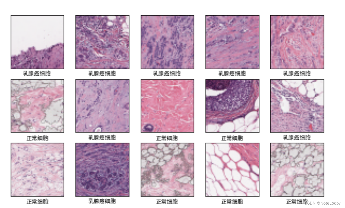
4. 数据可视化

plt.figure(figsize=(10, 8))  # 图形的宽为10高为5
plt.suptitle("数据展示")class_names = ["乳腺癌细胞","正常细胞"]for images, labels in train_ds.take(1):for i in range(15):plt.subplot(4, 5, i + 1)plt.xticks([])plt.yticks([])plt.grid(False)# 显示图片plt.imshow(images[i])# 显示标签plt.xlabel(class_names[labels[i]-1])plt.show()

三、构建模型

import tensorflow as tfmodel = tf.keras.Sequential([tf.keras.layers.Conv2D(filters=16,kernel_size=(3,3),padding="same",activation="relu",input_shape=[img_width, img_height, 3]),tf.keras.layers.Conv2D(filters=16,kernel_size=(3,3),padding="same",activation="relu"),tf.keras.layers.MaxPooling2D((2,2)),tf.keras.layers.Dropout(0.5),tf.keras.layers.Conv2D(filters=16,kernel_size=(3,3),padding="same",activation="relu"),tf.keras.layers.MaxPooling2D((2,2)),tf.keras.layers.Conv2D(filters=16,kernel_size=(3,3),padding="same",activation="relu"),tf.keras.layers.MaxPooling2D((2,2)),tf.keras.layers.Flatten(),tf.keras.layers.Dense(2, activation="softmax")
])
model.summary()

Model: "sequential"
_________________________________________________________________
Layer (type)                 Output Shape              Param #   
=================================================================
conv2d (Conv2D)              (None, 50, 50, 16)        448       
_________________________________________________________________
conv2d_1 (Conv2D)            (None, 50, 50, 16)        2320      
_________________________________________________________________
max_pooling2d (MaxPooling2D) (None, 25, 25, 16)        0         
_________________________________________________________________
dropout (Dropout)            (None, 25, 25, 16)        0         
_________________________________________________________________
conv2d_2 (Conv2D)            (None, 25, 25, 16)        2320      
_________________________________________________________________
max_pooling2d_1 (MaxPooling2 (None, 12, 12, 16)        0         
_________________________________________________________________
conv2d_3 (Conv2D)            (None, 12, 12, 16)        2320      
_________________________________________________________________
max_pooling2d_2 (MaxPooling2 (None, 6, 6, 16)          0         
_________________________________________________________________
flatten (Flatten)            (None, 576)               0         
_________________________________________________________________
dense (Dense)                (None, 2)                 1154      
=================================================================
Total params: 8,562
Trainable params: 8,562
Non-trainable params: 0
_________________________________________________________________

四、编译

model.compile(optimizer="adam",loss='sparse_categorical_crossentropy',metrics=['accuracy'])

五、训练模型

from tensorflow.keras.callbacks import ModelCheckpoint, Callback, EarlyStopping, ReduceLROnPlateau, LearningRateSchedulerNO_EPOCHS = 100
PATIENCE  = 5
VERBOSE   = 1# 设置动态学习率
annealer = LearningRateScheduler(lambda x: 1e-3 * 0.99 ** (x+NO_EPOCHS))# 设置早停
earlystopper = EarlyStopping(monitor='loss', patience=PATIENCE, verbose=VERBOSE)# 
checkpointer = ModelCheckpoint('best_model.h5',monitor='val_accuracy',verbose=VERBOSE,save_best_only=True,save_weights_only=True)

train_model  = model.fit(train_ds,epochs=NO_EPOCHS,verbose=1,validation_data=val_ds,callbacks=[earlystopper, checkpointer, annealer])

六、评估模型

1. Accuracy与Loss图

acc = train_model.history['accuracy']
val_acc = train_model.history['val_accuracy']loss = train_model.history['loss']
val_loss = train_model.history['val_loss']epochs_range = range(len(acc))plt.figure(figsize=(12, 4))
plt.subplot(1, 2, 1)plt.plot(epochs_range, acc, label='Training Accuracy')
plt.plot(epochs_range, val_acc, label='Validation Accuracy')
plt.legend(loc='lower right')
plt.title('Training and Validation Accuracy')plt.subplot(1, 2, 2)
plt.plot(epochs_range, loss, label='Training Loss')
plt.plot(epochs_range, val_loss, label='Validation Loss')
plt.legend(loc='upper right')
plt.title('Training and Validation Loss')
plt.show()

2. 混淆矩阵

from sklearn.metrics import confusion_matrix
import seaborn as sns
import pandas as pd# 定义一个绘制混淆矩阵图的函数
def plot_cm(labels, predictions):# 生成混淆矩阵conf_numpy = confusion_matrix(labels, predictions)# 将矩阵转化为 DataFrameconf_df = pd.DataFrame(conf_numpy, index=class_names ,columns=class_names)  plt.figure(figsize=(8,7))sns.heatmap(conf_df, annot=True, fmt="d", cmap="BuPu")plt.title('混淆矩阵',fontsize=15)plt.ylabel('真实值',fontsize=14)plt.xlabel('预测值',fontsize=14)

val_pre   = []
val_label = []for images, labels in val_ds:#这里可以取部分验证数据（.take(1)）生成混淆矩阵for image, label in zip(images, labels):# 需要给图片增加一个维度img_array = tf.expand_dims(image, 0) # 使用模型预测图片中的人物prediction = model.predict(img_array)val_pre.append(class_names[np.argmax(prediction)])val_label.append(class_names[label])

plot_cm(val_label, val_pre)

3. 各项指标评估

from sklearn import metricsdef test_accuracy_report(model):print(metrics.classification_report(val_label, val_pre, target_names=class_names)) score = model.evaluate(val_ds, verbose=0)print('Loss function: %s, accuracy:' % score[0], score[1])test_accuracy_report(model)

             precision    recall  f1-score   support乳腺癌细胞       0.92      0.90      0.91      1339正常细胞       0.91      0.92      0.91      1341accuracy                           0.91      2680macro avg       0.91      0.91      0.91      2680
weighted avg       0.91      0.91      0.91      2680Loss function: 0.22688131034374237, accuracy: 0.9138059616088867

pport

   乳腺癌细胞       0.92      0.90      0.91      1339正常细胞       0.91      0.92      0.91      1341accuracy                           0.91      2680

macro avg 0.91 0.91 0.91 2680
weighted avg 0.91 0.91 0.91 2680

Loss function: 0.22688131034374237, accuracy: 0.9138059616088867