引言

本文开始从零实现GPT1做一个小说续写器，即只需要给出一些文本，让模型帮你续写，主要内容包含：

• 模型编写
• 训练适配小说的中文分词器
• 将小说按固定大小拆分生成数据集
• 拆分训练/测试集
• 训练
• 体验小说续写效果

同时结合HuggingFace的transformers，可以将处理好的数据集、训练好的分词器和模型上传到HuggingFace Hub。

本文主要实现模型编写，剩下的内容请见下篇文章。

模型架构

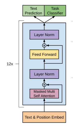
GPT模型架构如上图所示，由多层Tranformer Decoder组成的单向语言模型，是Tranformer的一个变种。它的Transformer Block比较简单，由两个子层组成，第一个子层输入上应用一个多头注意力层，输入和输出经过残差连接，紧着的是一个层归一化；第二个子层是前馈层、残差连接和层归一化。

整个GPT可以分为三部分：

1. 输入层
2. 编码层
3. 输出层

输入层计算出Transformer Block的输入表示；编码层经过叠加的多层Transformer Block进行编码；最后输出层应用Softmax计算输出标记的分布。

其训练过程包含两个阶段：无监督预训练和有监督微调。

无监督阶段可以在大规模文本语料上学习一个高容量的语言模型，然后可以根据下游具体任务进行微调。

无监督预训练

GPT是一个单向模型，也是仅解码器模型(Decoder Only)，即只能自左向右(或反之)对文本序列建模，采用的是Transformer的解码器结构，同时引入了同样的解码策略保证输入文本每个位置只能依赖当前和过去时刻的信息。

给定文本序列$w=w_1{w}_2\cdots w_n$，首先通过输入层将其编码成稠密向量：
$${u\text{u}u}_i={u\text{u}u}_i^e+{u\text{u}u}_i^p\text{\hspace{1em}(1)}$$
输入层由两个子层组成：词嵌入层和位置编码层。

其中${u\text{u}u}_i^e$是$w_i$经过词嵌入层得到的词向量；${u\text{u}u}_i^p$是$w_i$的经过位置编码层得到的位置向量；${u\text{u}u}_i$为第$i$个位置的标记经过输入层后的输出。

GPT的位置编码和原始Transformer中固定的不同，它是一种可学习的位置编码。

经过输入层得到每个标记带位置信息的词嵌入表示序列$u\text{u}u={u\text{u}u}_1\cdots {u\text{u}u}_n$，接着将$u\text{u}u$输入GPT的编码层，编码层由$L$个Transformer Block组成，每一层的Block都能计算出带有上下文信息的向量表示，经过多层编码后，能得到更复杂、强大的向量表示，计算过程为：
$${h\text{h}h}^l={\text{transformer\_block}}^l({h\text{h}h}^{l-1})\forall l\in [1,L]\text{\hspace{1em}(2)}$$
其中我们令${h\text{h}h}^0=u\text{u}u$，即输入层计算出来的输出；${h\text{h}h}^l\in {\mathbb{R}}^{d\times n}$表示由第$l$层计算出来的表示向量序列，$d$是模型隐藏层维度，$n$为序列长度；$L$为总层数。

而输出层基于最后一层的向量表示${h\text{h}h}^L$计算每个位置上输出标记的概率分布：
$$P(w_i|w_1,\cdots ,w_{i-1})=\text{softmax}({W\text{W}W}^e{h\text{h}h}_i^L)\text{\hspace{1em}(3)}$$
这里${W\text{W}W}^e\in {\mathbb{R}}^{|\mathbb{V}|\times d}$是词向量矩阵；$|\mathbb{V}|$为词表大小；注意这里${h\text{h}h}_i^L$的维度是$d\times 1$。

然后使用一个常规的语言建模目标优化$w$的最大似然估计：
$${\mathcal{L}}^{\text{PT}}=-\sum _i\log P(w_i|w_{i-k}\cdots w_{i-1};\Theta )\text{\hspace{1em}(4)}$$
这里的$k$是上下文窗口，根据前$k$个标记来预测当前标记；$\Theta$表示模型参数。

这就是预训练(pretrain)阶段的损失函数。

有监督微调

无监督预训练使得模型具有一定的通用语义表示能力，下游任务微调目的使通用语义表示可以适配不同具体的下游任务。

微调一般需要利用有标签数据集进行，假设一个有标签数据集$\mathcal{C}$，其中每个样本包含一个输入序列$x=x_1{x}_2\cdots x_n$和一个输出标签$y$。

将$x$输入给预训练好的模型，我们用最后一层Transformer Block的最后一个位置的输出${h\text{h}h}_n^L$来进行预测，具体地可以接一个全连接层结合$\text{softmax}$函数得到预测标签的概率分布：
$$p(y|x_1\cdots x_n)=\text{softmax}({h\text{h}h}_n^L{W\text{W}W}^y)\text{\hspace{1em}(5)}$$
其中${W\text{W}W}^y\in {\mathbb{R}}^{d\times c}$为全连接层参数；$c$为标签个数。通过对整个标注数据集进行优化，我们又可以得到微调目标函数：
$${\mathcal{L}}^{\text{FT}}(\mathcal{C})=-\sum _{(x,y)}\log P(y|x_1\cdots x_n)\text{\hspace{1em}(6)}$$
在下游任务微调过程中，如果仅针对微调目标进行优化，很可能会使模型遗忘预训练阶段所学习到的通用语义表示知识，从而损失模型的通用性和泛化能力，即灾难性遗忘(Catastrophic Forgetting)。因此将语言建模任务作为一个辅助目标函数加到微调阶段可以有助于学习，具体地，我们优化下面的目标函数：
$$\mathcal{L}={\mathcal{L}}^{\text{FT}}(\mathcal{C})+\lambda {\mathcal{L}}^{\text{PT}}(\mathcal{C})\text{\hspace{1em}(7)}$$
其中$\lambda$是用于平衡这两个目标函数的权重，可以取值$0.5$。

模型实现

本节我们开始从零实现GPT，有了上篇文章从零实现Transformer的基础，实现GPT也不是太难。

本次实现参考了HuggingFace的源码，使得我们后面可以很容易的应用HuggingFace实现的GPT。

开始之前，我们回顾下GPT论文中实现细节。

实现细节

模型设定

• 模型主要沿用原始的Transformer；
• 训练了一个带掩码自注意力头(状态维度768,12个头)的12层仅解码器的Transformer；
• 对于位置感知的前馈网络，使用3072作为内部隐状态维度；
• 使用Adam优化器和最大学习率2.5e-4；
• 学习率在前2000步内逐渐从0开始线性地增加，然后使用余弦调度器降低到0；
• 在批大小为64的长度为512的序列样本上训练；
• 由于模型中广泛使用层归一化，因此简单地(高斯)权重初始化；
• 使用了一个包含40000个合并的字节对编码(BPE)词表；
• 应用残差、嵌入和注意力的Dropout为0.1进行正则化；
• 采用了修改版的L2正则化；
• 对所有非偏置或增益权重使用$w=0.01$；
• 对于激活函数，使用GELU；
• 使用了学习的位置嵌入，而不是原始工作中的正弦版本。

微调细节

• 基本重复使用了无监督预训练的超参数设置；
• 在分类器中添加了0.1的Dropout；
• 对于大多数任务，使用6.25e-5的学习率和32的批量大小；
• 模型可以快速微调，大多数情况下3个epoch就足够了；
• 使用线性学习率衰减调度，并在0.2%的训练期上进行预热；
• 两个损失函数间的$\lambda$设置为0.5；

我们按照从下至上的原则依次实现。

输入层

上面我们知道，输入层由两个子层：词嵌入层和可学习的位置编码层组成，那就非常简单了，实际上就是两个嵌入层：

te=nn.Embedding(vocab_size, embed_dim )  # token emebedding 词嵌入层
pe=nn.Embedding(max_positions, embed_dim ) # 位置编码层

vocab_size是词表大小；embed_dim是模型嵌入大小；max_positions是最大可学习位置长度。

编码层

编码层由$L$层Transformer Block组成，每个Block的结构如上图所示。我们依次实现。

GELU

激活函数使用GELU而不是RELU，我们来看下GELU的图像(蓝线)：

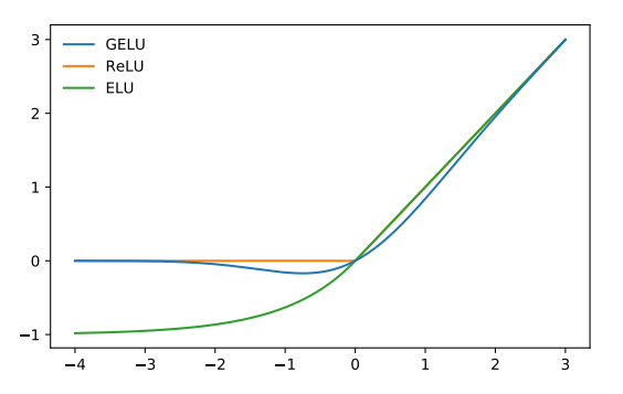
其近似公式为：
$$0.5x(1+\tanh [\sqrt{2/\pi }(x+0.044715x^3)])\text{\hspace{1em}(8)}$$
从图像可以看到，相比RELU和ELU，GELU有以下优势：

• 平滑性： GELU函数在整个输入范围内是光滑的，而ReLU在负数部分不是光滑的(其导数为0)，虽然ELU在负数部分是光滑的，但变化不够平滑。这使得GELU更容易优化；
• 高性能： GELU函数表现出比ReLU和ELU更好的性能；
• 非线性：GELU函数是非线性的，引入类似sigmoid函数的变换，使得GELU函数的输出可以落在一个更广的范围内，有助于加速模型的收敛；

按照公式实现即可：

class GELU(nn.Module):def forward(self, x: Tensor) -> Tensor:return (0.5* x* (1.0+ torch.tanh(math.sqrt(2.0 / math.pi)* (input + 0.044715 * torch.pow(input, 3.0)))))

但是为了速度快一点，我们应用Pytorch内建的torch.nn.functional.gelu。

一维卷积层

OpenAI GPT的作者把Transformer中的线性层命名为一维卷积，因为它们的操作是相等的(卷积的filter大小为1)。

我们通过图片来直观理解一下， https://ezyang.github.io/convolution-visualizer/ 提供了一个很好地可视化页面。

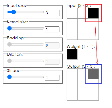
实际上filter大小为1的一维卷积就是让输入中每个位置与权重相乘(即序列长度维度上是并行独立计算的)，通过out_channels控制输出维度。

我们可以通过代码验证一下：

import torch
import torch.nn as nnembed_dim = 10
seq_len = 3
batch_size = 2
hidden_size = 5
# 定义输入数据，表示
x = torch.randn(batch_size, seq_len, embed_dim)# 定义前馈网络
fc = torch.nn.Linear(embed_dim, hidden_size)# 定义一维卷积核
conv = torch.nn.Conv1d(embed_dim, hidden_size, kernel_size=1)# 设置前馈网络和一维卷积核的参数相同
conv.weight = nn.Parameter(fc.weight.reshape(hidden_size, embed_dim, 1))
conv.bias = fc.bias# 计算前馈网络和一维卷积的输出结果
fc_output = fc(x)
x_conv = x.permute(0, 2, 1)
conv_output = conv(x_conv)# 比较输出结果是否相同
conv_output = conv_output.permute(0, 2, 1)print(torch.allclose(fc_output, conv_output))

True

所以它只是一个命名上的技巧，实际上实现起来还是通过前馈网络，不过与FeedForward中权重参数的维度位置相反，我们先看这里Conv1D的实现：

class Conv1D(nn.Module):def __init__(self, in_features: int, out_features: int) -> None:"""1D-convolutional layer as defined by Radford et al. for OpenAI GPT.Args:in_features (int): the number of input features.out_features (int): the number of output features."""super().__init__()self.out_features = out_featuresself.weight = nn.Parameter(torch.empty(in_features, out_features))self.bias = nn.Parameter(torch.zeros(out_features))nn.init.normal_(self.weight, std=0.02)def forward(self, x: Tensor) -> Tensor:"""Args:x (Tensor): (batch_size, seq_len, embed_dim)Returns:Tensor: (batch_size, seq_len, out_features)"""# size_out (batch_size, seq_len, out_features)size_out = x.size()[:-1] + (self.out_features,)# self.bias + x @ self.weight# x -view-> (batch_size *  seq_len,embed_dim)# (batch_size * seq_len,embed_dim) x (embed_dim, out_features)# -> (batch_size * seq_len, out_features)x = torch.addmm(self.bias, x.view(-1, x.size(-1)), self.weight)# x (batch_size, seq_len, out_features)x = x.view(size_out)return x

而Pytorch中FeedForward的实现(去掉一些细节)为：

class Linear(Module):def __init__(self, in_features: int, out_features: int, bias: bool = True,device=None, dtype=None) -> None:super(Linear, self).__init__()self.in_features = in_featuresself.out_features = out_featuresself.weight = Parameter(torch.empty((out_features, in_features), **factory_kwargs))if bias:self.bias = Parameter(torch.empty(out_features, **factory_kwargs))else:self.register_parameter('bias', None)self.reset_parameters()def reset_parameters(self) -> None:init.kaiming_uniform_(self.weight, a=math.sqrt(5))if self.bias is not None:fan_in, _ = init._calculate_fan_in_and_fan_out(self.weight)bound = 1 / math.sqrt(fan_in) if fan_in > 0 else 0init.uniform_(self.bias, -bound, bound)def forward(self, input: Tensor) -> Tensor:return F.linear(input, self.weight, self.bias)

我们来看应用Conv1D的例子：

embed_dim = 768
conv1d = Conv1D(embed_dim, embed_dim * 3)
# (batch_size, seq_len, embed_dim)
x = torch.rand(2, 5, embed_dim)
# (batch_size, seq_len, embed_dim * 3)
x = conv1d(x)
print(x.shape)

torch.Size([2, 5, 2304])

前馈层

那么就可以应用上面的一维卷积来实现前馈层了：

from torch.nn import functional as Fclass MLP(nn.Module):def __init__(self, config: GPTConfig) -> None:super().__init__()embed_dim = config.n_embdself.c_fc = Conv1D(embed_dim, embed_dim * 4)self.c_proj = Conv1D(embed_dim * 4, embed_dim)self.act = F.geluself.dropout = nn.Dropout(config.dropout)def forward(self, x: Tensor) -> Tensor:"""Args:x (Tensor): (batch_size, seq_len, embed_dim)Returns:Tensor: (batch_size, seq_len, embed_dim)"""# h (batch_size, seq_len, embed_dim * 4)h = self.act(self.c_fc(x))# h (batch_size, seq_len, embed_dim)h = self.c_proj(h)return self.dropout(h)

层归一化

层归一化这里我们直接使用Pytorch内建的torch.nn.LayerNorm。

掩码多头注意力

下面我们来实现掩码多头注意力，GPT中的注意力需要防止泄露未来的信息，因此自带一个下三角矩阵。

这可以通过以下代码实现：

import torchn_positions = 10torch.tril(torch.ones(n_positions, n_positions))

tensor([[1., 0., 0., 0., 0., 0., 0., 0., 0., 0.],[1., 1., 0., 0., 0., 0., 0., 0., 0., 0.],[1., 1., 1., 0., 0., 0., 0., 0., 0., 0.],[1., 1., 1., 1., 0., 0., 0., 0., 0., 0.],[1., 1., 1., 1., 1., 0., 0., 0., 0., 0.],[1., 1., 1., 1., 1., 1., 0., 0., 0., 0.],[1., 1., 1., 1., 1., 1., 1., 0., 0., 0.],[1., 1., 1., 1., 1., 1., 1., 1., 0., 0.],[1., 1., 1., 1., 1., 1., 1., 1., 1., 0.],[1., 1., 1., 1., 1., 1., 1., 1., 1., 1.]])

先来看一下初始化方法：

def __init__(self, config: GPTConfig, scale: bool = False) -> None:super().__init__()self.n_embd = config.n_embdassert config.n_embd % config.n_head == 0self.scale = scaleself.n_head = config.n_headself.c_attn = Conv1D(self.n_embd, self.n_embd * 3)self.c_proj = Conv1D(self.n_embd, self.n_embd)# use flash attention or notself.flash = hasattr(torch.nn.functional, "scaled_dot_product_attention")if not self.flash:self.register_buffer("bias",torch.tril(torch.ones(config.n_positions, config.n_positions)).view(1, 1, config.n_positions, config.n_positions),persistent=False,  # will not be saved alongside parameters)self.attn_dropout = nn.Dropout(config.dropout)self.proj_dropout = nn.Dropout(config.dropout)

主要操作是调用上面实现的Conv1D，c_attn这样定义为了可以同时计算query,key,value所有的头，因为在GPT中只有自注意力，由同一个输入计算出不同的query,key,value值，所以可以这样实现。

如果还Pytorch2.0及以上的版本，则torch.nn.functional有scaled_dot_product_attention函数，它利用Flash Attention高效计算。

否则通过register_buffer将下三角矩阵注册为buffer，并且不需要随着模型参数保存，转换为(1,1,n_positions,n_positions)的形状是为了适配批次和多个头。

接下来实现forward()函数：

 def forward(self, x: Tensor, output_attentions: bool = False) -> list[Tensor]:"""Args:x (Tensor): (batch_size, seq_len, n_embd)Returns:Tensor: (batch_size, seq_len, n_embd) attn_outputTensor(optional): (batch_size, n_head, seq_len, seq_len) attn_weights"""# calculate query, key ,value for all heads in batch# x (batch_size, seq_len, n_embd * 3)x = self.c_attn(x)#  query, key, value (batch_size, seq_len, n_embd)query, key, value = x.split(self.n_embd, dim=2)# query (batch_size,  n_head, seq_len, n_embd / n_head)query = self.split_heads(query)# key (batch_size, n_head, n_embd / n_head, seq_len)key = self.split_heads(key, is_key=True)# value (batch_size,  n_head, seq_len, n_embd / n_head)value = self.split_heads(value)# attn_output (batch_size,  n_head, seq_len, n_embd / n_head)attn_outputs = self._attn(query, key, value, output_attentions)attn_output = attn_outputs[0]# output (batch_size, seq_len, n_embd)output = self.merge_heads(attn_output)# (batch_size, seq_len, n_embd)output = self.c_proj(output)output = self.proj_dropout(output)outputs = [output] + attn_outputs[1:]return outputs

主要过程为：

1. 通过c_attn一次计算出所有头的q,k,v值，得到的输出维度是(batch_size, seq_len, n_embd * 3)；

2. 调用split在最后一个维度上将输出拆分成q,k,v矩阵；

3. 在q,k,v上分别调用split_heads()拆分成n_head个头；

4. 传入q,k,v调用_attn()得到注意力计算结果；

5. 调用merge_heads()拼接多头注意力的结果；

6. 最后经过一个线性变换c_proj；

split_heads其实就是一个变形(view)操作：

    def split_heads(self, x: Tensor, is_key: bool = False) -> Tensor:"""Args:x (Tensor): (batch_size, seq_len, n_embd)is_key (bool, optional): is key or not. Defaults to False.Returns:Tensor: (batch_size, n_head, n_embd / n_head, seq_len) if is_key = True ,else (batch_size,  n_head, seq_len, n_embd / n_head)"""# (batch_size, seq_len, n_head, n_embd / n_head)new_shape = x.size()[:-1] + (self.n_head, x.size(-1) // self.n_head)# x (batch_size, seq_len, n_head, n_embd / n_head)x = x.view(*new_shape)if is_key:# (batch_size, n_head, n_embd / n_head, seq_len)return x.permute(0, 2, 3, 1)# (batch_size,  n_head, seq_len, n_embd / n_head)return x.permute(0, 2, 1, 3)

接着就是核心的注意力操作_attn：

def _attn(self,q: Tensor,k: Tensor,v: Tensor,attention_mask: Tensor = None,output_attentions: bool = False,
) -> list[Tensor]:"""Args:q (Tensor): (batch_size,  n_head, seq_len, n_embd / n_head)k (Tensor): (batch_size, n_head, n_embd / n_head, seq_len)v (Tensor): (batch_size,  n_head, seq_len, n_embd / n_head)Returns:Tensor: (batch_size,  n_head, seq_len, n_embd / n_head) attn_outputTensor(optional): (batch_size, n_head, seq_len, seq_len) attn_weights"""if self.flash:# 使用flash attentionattn_output = torch.nn.functional.scaled_dot_product_attention(q,k,v,attn_mask=None,dropout_p=self.attn_dropout.p if self.training else 0,is_causal=True, # 传入True的话attn_mask必须为None)weights = Noneelse:# scores (batch_size,  n_head, seq_len, seq_len)scores = torch.matmul(q, k)if self.scale:scores = scores / math.sqrt(v.size(-1))# scores = scores.masked_fill(#    self.bias[:, :, : scores.size(-2), : scores.size(-1)] == 0, float("-inf")# )bias = self.bias[:, :, : scores.size(-2), : scores.size(-1)]# more efficient than masked_fillscores = scores * bias + -1e9 * (1 - bias)# weights (batch_size,  n_head, seq_len, seq_len)weights = self.attn_dropout(F.softmax(scores, dim=-1))if attention_mask is not None:weights = weights + attention_maskdel scores# attn_output (batch_size,  n_head, seq_len, n_embd / n_head)attn_output = torch.matmul(weights, v)outputs = [attn_output]if output_attentions:outputs.append(weights)return outputs

与上篇文章Transformer中实现的注意力计算几乎没有变化，对注意力得分scores进行一个下三角掩码，这里实现的时候采用比masked_fill更高效的乘法和加法的方式。

然后调用softmax得到注意力权重，与v矩阵相乘得到最后的注意力输出。

接下来通过merge_heads拼接多个注意力头的结果：

    def merge_heads(self, x: Tensor) -> Tensor:"""Args:x (Tensor):  (batch_size,  n_head, seq_len, n_embd / n_head)Returns:Tensor: (batch_size, seq_len, n_embd)"""# x (batch_size,  seq_len, n_head, n_embd / n_head)x = x.permute(0, 2, 1, 3).contiguous()# (batch_size, seq_len, n_embd)new_shape = x.size()[:-2] + (x.size(-2) * x.size(-1),)return x.view(*new_shape)

其实也是变形操作。最后经过一次线性投影。

此时模型还未进行过非线性操作，为了增强表达能力，通过前馈层引入非线性操作。

实现Block

class Block(nn.Module):def __init__(self, config: GPTConfig, scale: bool = False) -> None:super().__init__()n_embd = config.n_embdself.attn = Attention(config, scale)self.ln_1 = nn.LayerNorm(n_embd)self.mlp = MLP(config)self.ln_2 = nn.LayerNorm(n_embd)def forward(self, x: Tensor, attention_mask: Tensor = None, output_attentions: bool = False) -> Tensor:"""_summary_Args:x (Tensor): (batch_size, seq_len, n_embd)attention_mask (Tensor, optional)output_attentions (bool, optional)Returns:Tensor: (batch_size, seq_len, n_embd) block outputTensor(optional): (batch_size, n_head, seq_len, seq_len) attn_weights"""attn_outputs = self.attn(x, attention_mask, output_attentions)# a : attention output (batch_size, n_head, seq_len, n_embd / n_head)a = attn_outputs[0]# resident connection and layer norm# n (batch_size, seq_len, n_embd)n = self.ln_1(x + a)# m (batch_size, seq_len, n_embd)m = self.mlp(n)# resident connection and layer norm# h (batch_size, seq_len, n_embd)h = self.ln_2(n + m)outputs = [h] + attn_outputs[1:]return outputs

Block的实现就很简单，按照架构图实现即可。这里的attention_mask是用于对对填充Token进行掩码。

实现GPT模型

首先我们要继承transformers的PreTrainedModel，最终可以将训练好的模型上传到HuggingFace的Hub上分享给大家。

在这之前我们需要编写自定义配置，包含构建模型所需的所有信息：

from transformers import PretrainedConfigclass GPTConfig(PretrainedConfig):model_type = "openai-gpt" # 这个就是openai的gpt1def __init__(self,vocab_size=5000,n_positions=1024,n_embd=768,n_layer=12,n_head=12,dropout=0.1,initializer_range=0.02,**kwargs) -> None:"""Args:vocab_size (int, optional): vocabulary size. Defaults to 5000.n_positions (int, optional): the maximum sequence length that this model might ever be used with. Defaults to 1024.n_embd (int, optional): dimensionality of the embeddings and hidden states. Defaults to 768.n_layer (int, optional): number of hidden layers. Defaults to 12.n_head (int, optional): number of attention heads for each attention layer. Defaults to 12.dropout (float, optional): the dropout probability. Defaults to 0.1.initializer_range (tuple, optional): the standard deviation of the truncated_normal_initializer for initializing all weight matrices. Defaults to (0.02,)."""self.vocab_size = vocab_sizeself.n_positions = n_positionsself.n_embd = n_embdself.n_layer = n_layerself.n_head = n_headself.dropout = dropoutself.initializer_range = initializer_rangesuper().__init__(**kwargs)

编写自定义配置需要注意三点：

• 继承自PretrainedConfig；
• __init__方法中必须存在接收任何参数的kwargs；
• 这些kwargs需要传递给父类的__init__方法；

通过继承我们可以获得Transformers库的额外功能，另外两个条件是接收PretrainedConfig额外的字段。

有了配置后，我们继续编写GPT模型，同样继承类似的PreTrainedModel。先定义一个基类，主要传入配置文件、定义参数初始化方法。

class GPTPreTrainedModel(PreTrainedModel):"""An abstract class to handle weights initialization and a simple interface for downloading and loading pretrainedmodels."""config_class = GPTConfigbase_model_prefix = "transformer"def __init__(self, config: PretrainedConfig):super().__init__(config)def _init_weights(self, module):if isinstance(module, (nn.Linear, Conv1D)):module.weight.data.normal_(mean=0.0, std=self.config.initializer_range)if module.bias is not None:module.bias.data.zero_()elif isinstance(module, nn.Embedding):module.weight.data.normal_(mean=0.0, std=self.config.initializer_range)if module.padding_idx is not None:module.weight.data[module.padding_idx].zero_()elif isinstance(module, nn.LayerNorm):module.bias.data.zero_()module.weight.data.fill_(1.0)

现在就可以定义我们的GPT模型了：

class GPTModel(GPTPreTrainedModel):def __init__(self, config: GPTConfig) -> None:super().__init__(config)self.config = configself.tokens_embed = nn.Embedding(config.vocab_size, config.n_embd)self.positions_embed = nn.Embedding(config.n_positions, config.n_embd)self.dropout = nn.Dropout(config.dropout)self.h = nn.ModuleList([Block(config, scale=True) for _ in range(config.n_layer)])self.register_buffer("position_ids", torch.arange(config.n_positions), persistent=False)self.post_init()

继承自上面定义的GPTPreTrainedModel，接收配置类。这里负责定义词嵌入和位置编码，对于这个可学习的位置编码，还需要定义表示位置的序列，从0到最大位置，即position_ids。

然后堆叠多层Block，最后调用self.post_init()，这是PreTrainedModel中为我们实现的一个方法，它实际会调用我们自己定义的_init_weights。

再来看前向传播方法：

def forward(self,input_ids: torch.LongTensor,attention_mask: Tensor = None,output_attentions: bool = False,output_hidden_states: bool = False,return_dict: bool = False,
) -> Union[Tuple[torch.Tensor], BaseModelOutput]:"""Args:input_ids (torch.LongTensor): (batch_size, seq_len)output_attentions (bool, optional): whether or not to return the attentions tensors of all attention layers. Defaults to False.output_hidden_states (bool, optional): whether or not to return the hidden states of all layers. Defaults to False.return_dict (bool, optional): whether or not to return a ModelOutput instead of a plain tuple. Defaults to False.Returns:Union[Tuple[torch.Tensor], BaseModelOutput]: tuple or BaseModelOutput"""input_shape = input_ids.size()inputs_embeds = self.tokens_embed(input_ids)# generate position idsposition_ids = self.position_ids[None, : input_shape[-1]]position_embeds = self.positions_embed(position_ids)hidden_states = inputs_embeds + position_embedshidden_states = self.dropout(hidden_states)all_attentions = () if output_attentions else Noneall_hidden_states = () if output_hidden_states else Nonefor _, block in enumerate(self.h):if output_hidden_states:all_hidden_states = all_hidden_states + (hidden_states,)outputs = block(hidden_states, attention_mask, output_attentions)hidden_states = outputs[0]if output_attentions:all_attentions = all_attentions + (outputs[1],)# add last layerif output_hidden_states:all_hidden_states = all_hidden_states + (hidden_states,)if not return_dict:return tuple(vfor v in [hidden_states, all_hidden_states, all_attentions]if v is not None)return BaseModelOutput(last_hidden_state=hidden_states,hidden_states=all_hidden_states,attentions=all_attentions,)

这样我们的GPT编码层就实现好了。