在使用多目标跟踪算法时，接触到卡尔曼滤波，一直没时间总结下，现在来填坑。

1. 背景知识

在理解卡尔曼滤波前，有几个概念值得考虑下：时序序列模型，滤波，线性动态系统

1. 时间序列模型

时间序列模型都可以用如下示意图表示：

这个模型包含两个序列，一个是黄色部分的状态序列，用X表示，一个是绿色部分的观测序列（又叫测量序列、证据序列、观察序列，不同的书籍有不同的叫法，在这里统一叫观测序列。）用Y表示。状态序列反应了系统的真实状态，一般不能被直接观测，即使被直接观测也会引进噪声；观测序列是通过测量得到的数据，它与状态序列之间有规律性的联系。

上面序列中，假设初始时间为t1t1, 则X1,Y1X1,Y1是t1t1时刻的状态值和观测值，X2,Y2X2,Y2是t2t2时刻的状态值和观测值…，即随着时间的流逝，序列从左向右逐渐展开。

常见的时间序列模型主要包括三个：隐尔马尔科夫模型，卡尔曼滤波，粒子滤波。

2. 滤波

时间序列模型中包括预测和滤波两步

• 预测：指用当前和过去的数据来求取未来的数据。对应上述序列图中，则是利用t1t1时刻X1,Y1X1,Y1的值，估计t2t2时刻X2X2值。
• 滤波：是用当前和过去的数据来求取当前的数据。对应上述序列图中，则是先通过上一步的预测步骤得到X2X2的一个预测值，再利用t2t2时刻Y2Y2的值对这个预测值进行纠正，得到最终的X2X2估计值。（通俗讲，就是通过X1X1预测一个值, 通过传感器测量一个值Y2Y2, 将两者进行融合得到最终的X2X2值）

3.线性动态系统

卡尔曼滤波又称为基于高斯过程的线性动态系统(Linear Dynamic System, LDS) , 这里的高斯是指：状态变量XtXt和观测变量YtYt都符合高斯分布；这里的线性是指：XtXt可以通过Xt−1Xt−1线性表示，YtYt可以通过XtXt线性表示；如果用数学表达式来表达这两层含义如下：

Xt=FXt−1+wt−1,wt−1∼N(0,Q)Xt=FXt−1+wt−1,wt−1∼N(0,Q)

上面表达式中F是一个矩阵，常称作状态转移矩阵，保证了XtXt和Xt−1Xt−1的线性关系(线性代数中，矩阵就是线性变换)；wt−1wt−1常称作噪声，其服从均值为0，方差为Q的高斯分布，保证了XtXt服从高斯分布(因为高斯分布加上一个常数后依然是高斯分布)。

同样的关于XtXt和YtYt,也可以得到如下表示, 其中矩阵H称作状态空间到观测空间的映射矩阵， rtrt称作噪声，其服从高斯分布：

Yt=HXt+rt,(rt∼N(0,R))Yt=HXt+rt,(rt∼N(0,R))

参考：https://zhuanlan.zhihu.com/p/139215491

2. 卡尔曼滤波理论知识

关于卡尔曼滤波的理论知识有很多文章讲的很好，参考下面的两个链接

https://zhuanlan.zhihu.com/p/25598462

http://www.bzarg.com/p/how-a-kalman-filter-works-in-pictures/#mjx-eqn-gaussequiv

这里简单总结下用得到数学表达式，方便实际编程时查阅和理解：

2.1 状态序列的预测

在时间序列模型图中，这一步表示的是, 在预测序列中，从Xt−1Xt−1到XtXt的预测步骤。

需要用到的变量含义如下：

• ^xkxk:状态变量
• ^PkPk: 状态变量的协方差矩阵
• FkFk:状态转移矩阵
• BkBk:控制矩阵
• μkμk:控制向量
• wkwk: 状态变量的噪声矩阵
• QkQk:协方差矩阵的噪声矩阵

数学表达式如下：

^xk=Fkxk−1+Bk→μk+wk^Pk=FkPk−1FTk+Qkx^k=Fkxk−1+Bkμ→k+wkP^k=FkPk−1FkT+Qk

2.2 状态序列到观测序列的转换

在时间序列模型图中，这一步表示的是, 从XtXt到YtYt的转换。

需要用到的变量含义如下：

• HkHk:状态空间到测量空间的映射矩阵
• ^xkxk: tktk时刻的状态变量
• ^PkPk: tktk时刻状态变量的协方差矩阵

映射后变量的均值和方差如下：

→μexpected=Hk^{xkΣexpected=Hk}PkHTkμ→expected=Hkx^{kΣexpected=HkP}kHkT

2.3 测量序列的滤波

在时间序列模型图中，这一步表示的是，测量值YtYt对预测值XtXt进行纠正，得到最终的状态向量XtXt

观测向量服从高斯分布, 假设其均值和协方差矩阵如下：

观测向量均值：→μmeasurement=→zk观测向量协方差矩阵:Σmeasurement=Rk观测向量均值：μ→measurement=z→k观测向量协方差矩阵:Σmeasurement=Rk

我们已经得到了状态序列的预测值，而且将其映射到了测量序列，也得到了测量序列的测量值，接来要做的就是将两者进行融合，由于两者都符合高斯分布，其融合过程就是两个高斯分布的混合

1. 高斯混合

单变量高斯分布方程：

N(x,μ,σ)=1σ√2πe−(x−μ)22σ2N(x,μ0,σ0)⋅N(x,μ1,σ1)?=N(x,μ′,σ′)(1)(1)N(x,μ,σ)=1σ2πe−(x−μ)22σ2N(x,μ0,σ0)⋅N(x,μ1,σ1)=?N(x,μ′,σ′)

两个单变量高斯分布混合：

μ′=μ0+k(μ1−μ0)σ′2=kσ12=σ02(1−k)其中，k=σ20σ20+σ21μ′=μ0+k(μ1−μ0)σ′2=kσ12=σ02(1−k)其中，k=σ02σ02+σ12

以上是单变量概率密度函数的计算结果，如果是多变量的，那么，就变成了协方差矩阵的形式：

K=Σ0(Σ0+Σ1)−1→μ′=→μ0+K(→μ1−→μ0)Σ′=KΣ1=Σ0(I−K)K=Σ0(Σ0+Σ1)−1μ→′=μ→0+K(μ→1−μ→0)Σ′=KΣ1=Σ0(I−K)

2. 预测值和测量值混合

预测值和测量值的均值和协方差如下：

预测值高斯分布：(μ0,Σ0)=(Hk^{xk,HkPkHTk)测量值高斯分布：(μ1,Σ1)=(zk,Rk)预测值高斯分布：(μ0,Σ0)=(Hkx}k,HkPkHkT)测量值高斯分布：(μ1,Σ1)=(zk,Rk)

预测值和测量值混合：

Hk^x′k=Hkxk+K(→zk−Hk^{xk)HkP′kHTk=HkPkHTk−KHkPkHTk其中，K称作卡尔曼增益：K=HkPkHTk(HkPkHTk+Rk)−1Hkx}k′=Hkx^{k+K(zk→−Hkx}k)HkPk′HkT=HkPkHkT−KHkPkHkT其中，K称作卡尔曼增益：K=HkPkHkT(HkPkHkT+Rk)−1

化简上述表达式，计算x′k,P′kxk′,Pk′，结果如下：(x′kxk′就是第k次卡尔曼预测结果, P′kPk′是该结果的协方差矩阵)

^x′k=xk+K′(→zk−Hk^{xk)P′k=Pk−K′HkPkK′=PkHTk(HkPkHTk+Rk)−1x}k′=x^{k+K′(zk→−Hkx}k)Pk′=Pk−K′HkPkK′=PkHkT(HkPkHkT+Rk)−1

最终，可以卡尔曼滤波流程图如下：

参考：https://zhuanlan.zhihu.com/p/142044672
https://zhuanlan.zhihu.com/p/158751412
https://zhuanlan.zhihu.com/p/58675854
https://leijiezhang001.github.io/卡尔曼滤波详解/
https://zhuanlan.zhihu.com/p/166342719

3. 卡尔曼滤波用于目标跟踪

对于一个小车，我们采用卡尔曼滤波来估计其位置，在进行估计的时候，有几个变量要进行定义和初始化。这里定义了六个变量的初始值：状态向量，状态向量协方差矩阵，状态向量协方差矩阵的噪声矩阵，动态转移矩阵，映射矩阵，测量值的协方差矩阵（假设小车是匀速运动，所以没有使用控制矩阵和控制变量）

1. 初始状态向量xx：（8x1的矩阵）

[xyahvxvyvavh]T[xyahvxvyvavh]T

其中对应含义和初始化值如下：

• (x,y)表示目标的中心点，a=w/h表示目标的宽高比，h表示目标的高度，初始化值为目标第一帧的位置
• v_x, v_y, v_a, v_h:表示对应变量随时间的变化率, 初始化值为0

2. 状态向量初始协方差矩阵PP：(8*8的矩阵， 这里如何设置，需要经验？)

⎡⎢ ⎢ ⎢ ⎢ ⎢ ⎢ ⎢ ⎢ ⎢ ⎢ ⎢ ⎢ ⎢ ⎢⎣151.2900000000151.29000000000.000100000000151.290000000059.090000000059.09000000000.000010000000059.09⎤⎥ ⎥ ⎥ ⎥ ⎥ ⎥ ⎥ ⎥ ⎥ ⎥ ⎥ ⎥ ⎥ ⎥⎦[151.2900000000151.29000000000.000100000000151.290000000059.090000000059.09000000000.000010000000059.09]

3.状态向量协方差矩阵的噪声矩阵QQ：(8*8的矩阵， 这里如何设置，需要经验？)

⎡⎢ ⎢ ⎢ ⎢ ⎢ ⎢ ⎢ ⎢ ⎢ ⎢ ⎢ ⎢ ⎢ ⎢⎣37.820000000037.82000000000.00010000000037.82000000000.59000000000.59000000000.00001000000000.59⎤⎥ ⎥ ⎥ ⎥ ⎥ ⎥ ⎥ ⎥ ⎥ ⎥ ⎥ ⎥ ⎥ ⎥⎦[37.820000000037.82000000000.00010000000037.82000000000.59000000000.59000000000.00001000000000.59]

4. 动态转移矩阵F：(8x8的矩阵)

⎡⎢ ⎢ ⎢ ⎢ ⎢ ⎢ ⎢ ⎢ ⎢ ⎢ ⎢ ⎢ ⎢ ⎢⎣1000100001000100001000100001000100001000000001000000001000000001⎤⎥ ⎥ ⎥ ⎥ ⎥ ⎥ ⎥ ⎥ ⎥ ⎥ ⎥ ⎥ ⎥ ⎥⎦[1000100001000100001000100001000100001000000001000000001000000001]

5. 映射矩阵H：（4x8的矩阵）

⎡⎢ ⎢ ⎢⎣10000000010000000010000000010000⎤⎥ ⎥ ⎥⎦[10000000010000000010000000010000]

6. 测量值的协方差矩阵RR：(4x4的矩阵, 这里如何设置，需要经验？)

⎡⎢ ⎢ ⎢⎣37.82000037.8200000.0001000037.82⎤⎥ ⎥ ⎥⎦[37.82000037.8200000.0001000037.82]

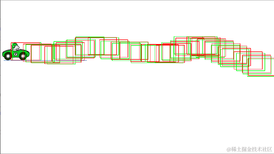
下面代码中，采用卡尔曼滤波，对小车的随机运动进行了估计，结果如图所示，绿色框表示小车的真实位置，红色框表示卡尔曼滤波的估计位置

# vim: expandtab:ts=4:sw=4
import numpy as np
import scipy.linalg
import cv2"""
Table for the 0.95 quantile of the chi-square distribution with N degrees of
freedom (contains values for N=1, ..., 9). Taken from MATLAB/Octave's chi2inv
function and used as Mahalanobis gating threshold.
"""
chi2inv95 = {1: 3.8415,2: 5.9915,3: 7.8147,4: 9.4877,5: 11.070,6: 12.592,7: 14.067,8: 15.507,9: 16.919}class KalmanFilter(object):"""A simple Kalman filter for tracking bounding boxes in image space.The 8-dimensional state spacex, y, a, h, vx, vy, va, vhcontains the bounding box center position (x, y), aspect ratio a, height h,and their respective velocities.Object motion follows a constant velocity model. The bounding box location(x, y, a, h) is taken as direct observation of the state space (linearobservation model)."""def __init__(self):ndim, dt = 4, 1.# Create Kalman filter model matrices.self._motion_mat = np.eye(2 * ndim, 2 * ndim)  # 初始化动态转移矩阵, shape(8, 8)for i in range(ndim):self._motion_mat[i, ndim + i] = dtself._update_mat = np.eye(ndim, 2 * ndim)   # 初始化映射矩阵，shape(4, 8)# Motion and observation uncertainty are chosen relative to the current# state estimate. These weights control the amount of uncertainty in# the model. This is a bit hacky.self._std_weight_position = 1. / 20self._std_weight_velocity = 1. / 160def initiate(self, measurement):"""Create track from unassociated measurement.Parameters----------measurement : ndarrayBounding box coordinates (x, y, a, h) with center position (x, y),aspect ratio a, and height h.Returns-------(ndarray, ndarray)Returns the mean vector (8 dimensional) and covariance matrix (8x8dimensional) of the new track. Unobserved velocities are initializedto 0 mean."""mean_pos = measurementmean_vel = np.zeros_like(mean_pos)mean = np.r_[mean_pos, mean_vel]   # 状态向量，shape(1, 8)std = [2 * self._std_weight_position * measurement[3],2 * self._std_weight_position * measurement[3],1e-2,2 * self._std_weight_position * measurement[3],10 * self._std_weight_velocity * measurement[3],10 * self._std_weight_velocity * measurement[3],1e-5,10 * self._std_weight_velocity * measurement[3]]covariance = np.diag(np.square(std))    # 状态向量协方差矩阵， shape(8, 8)return mean, covariancedef predict(self, mean, covariance):"""Run Kalman filter prediction step.Parameters----------mean : ndarrayThe 8 dimensional mean vector of the object state at the previoustime step.covariance : ndarrayThe 8x8 dimensional covariance matrix of the object state at theprevious time step.Returns-------(ndarray, ndarray)Returns the mean vector and covariance matrix of the predictedstate. Unobserved velocities are initialized to 0 mean."""std_pos = [self._std_weight_position * mean[3],self._std_weight_position * mean[3],1e-2,self._std_weight_position * mean[3]]std_vel = [self._std_weight_velocity * mean[3],self._std_weight_velocity * mean[3],1e-5,self._std_weight_velocity * mean[3]]motion_cov = np.diag(np.square(np.r_[std_pos, std_vel]))mean = np.dot(self._motion_mat, mean)  # 动态转移矩阵*状态向量covariance = np.linalg.multi_dot((self._motion_mat, covariance, self._motion_mat.T)) + motion_cov   # 动态转移矩阵*状态向量协方差矩阵 + 噪声矩阵return mean, covariancedef project(self, mean, covariance):"""Project state distribution to measurement space.Parameters----------mean : ndarrayThe state's mean vector (8 dimensional array).covariance : ndarrayThe state's covariance matrix (8x8 dimensional).Returns-------(ndarray, ndarray)Returns the projected mean and covariance matrix of the given stateestimate."""std = [self._std_weight_position * mean[3],self._std_weight_position * mean[3],1e-1,self._std_weight_position * mean[3]]innovation_cov = np.diag(np.square(std))mean = np.dot(self._update_mat, mean)   # 映射矩阵*状态向量covariance = np.linalg.multi_dot((self._update_mat, covariance, self._update_mat.T))return mean, covariance + innovation_cov         # 映射矩阵*状态向量 + 噪声矩阵def update(self, mean, covariance, measurement):"""Run Kalman filter correction step.Parameters----------mean : ndarrayThe predicted state's mean vector (8 dimensional).covariance : ndarrayThe state's covariance matrix (8x8 dimensional).measurement : ndarrayThe 4 dimensional measurement vector (x, y, a, h), where (x, y)is the center position, a the aspect ratio, and h the height of thebounding box.Returns-------(ndarray, ndarray)Returns the measurement-corrected state distribution."""projected_mean, projected_cov = self.project(mean, covariance)chol_factor, lower = scipy.linalg.cho_factor(projected_cov, lower=True, check_finite=False)    # Cholesky分解kalman_gain = scipy.linalg.cho_solve((chol_factor, lower), np.dot(covariance, self._update_mat.T).T,check_finite=False).T                             # 求解卡尔曼增益矩阵innovation = measurement - projected_meannew_mean = mean + np.dot(innovation, kalman_gain.T)    # 预测值和测量值融合后，新的状态向量new_covariance = covariance - np.linalg.multi_dot((kalman_gain, projected_cov, kalman_gain.T))        # 预测值和测量值融合后，新状态向量的协方差矩阵return new_mean, new_covariancedef gating_distance(self, mean, covariance, measurements,only_position=False):"""Compute gating distance between state distribution and measurements.A suitable distance threshold can be obtained from `chi2inv95`. If`only_position` is False, the chi-square distribution has 4 degrees offreedom, otherwise 2.Parameters----------mean : ndarrayMean vector over the state distribution (8 dimensional).covariance : ndarrayCovariance of the state distribution (8x8 dimensional).measurements : ndarrayAn Nx4 dimensional matrix of N measurements, each informat (x, y, a, h) where (x, y) is the bounding box centerposition, a the aspect ratio, and h the height.only_position : Optional[bool]If True, distance computation is done with respect to the boundingbox center position only.Returns-------ndarrayReturns an array of length N, where the i-th element contains thesquared Mahalanobis distance between (mean, covariance) and`measurements[i]`."""mean, covariance = self.project(mean, covariance)if only_position:mean, covariance = mean[:2], covariance[:2, :2]measurements = measurements[:, :2]cholesky_factor = np.linalg.cholesky(covariance)d = measurements - meanz = scipy.linalg.solve_triangular(cholesky_factor, d.T, lower=True, check_finite=False,overwrite_b=True)squared_maha = np.sum(z * z, axis=0)return squared_mahaif __name__ == "__main__":kf = KalmanFilter()img = cv2.imread("./car.png")m = np.array([108.5, 360.5, 1.618, 123])   # 小车的初始化测量值，分别表示小车的x_center, y_center, w/h, hmean_ini, covariance_ini = kf.initiate(m)  # 初始化卡尔曼的动态转移矩阵，映射矩阵for i in range(30):mean_pre, covariance_pre = kf.predict(mean_ini, covariance_ini)  # 预测状态变量dx = np.random.randint(0, 120)dy = np.random.randint(-30, 30)m = m + np.array([dx, dy, 0, 0])   # 随机向左，和上下移动cv2.rectangle(img, (int(m[0]-m[2]*m[3]/2), int(m[1]-m[3]/2)),(int(m[0]+m[2]*m[3]/2), int(m[1]+m[3]/2)), (0, 255, 0), 2)  # 用绿色框，绘制小车移动后的真实位置mean_upd, covariance_upd = kf.update(mean_pre, covariance_pre, m+np.random.randn(4))   # 利用测量值，更新状态变量mean_ini = mean_updcovariance_ini = covariance_upd# 用红色框，绘制小车移动后的估计位置cv2.rectangle(img, (int(mean_ini[0] - mean_ini[2] * mean_ini[3] / 2), int(mean_ini[1] - mean_ini[3] / 2)),(int(mean_ini[0] + mean_ini[2] * mean_ini[3] / 2), int(mean_ini[1] + mean_ini[3] / 2)), (0, 0, 255), 2)cv2.namedWindow("img", cv2.WINDOW_NORMAL)cv2.resizeWindow("img", 960, 540)cv2.imshow("img", img)cv2.waitKey(0)cv2.destroyAllWindows()